

Integration of 3D Seismic Attributes for Preliminary Shallow Geohazard Identification in Deep Water Exploration Area with No Well Data
HEAD OF TEAM : Prof. Sigit Sukmono
TEAM MEMBERS : Dona Sita Ambarsari, ST., MT.
Introduction
Drilling in the deep water is very challenging as the safety of drilling rigs and other installations could be threatened by the presence of shallow geohazards. These hazards are a global problem, and while the industry has matured in handling these problems, significant losses owing to the improper assessment of the geohazards prior to drilling have been widely reported (Campbell, 1999). In the Gulf of Mexico (GoM) alone, it was estimated that the associated losses continue to be more than $1.7 million per well (Dutta et al., 2010). ISO 17776 defines a hazard as a ‘potential source of harm’, thus shallow geohazards in the context of offshore drilling activ- ities can be defined as local and/or regional shallow geological features having potential to cause loss of life or damage to health, environment or assets. The geohazards characteristics vary from place to place depending on the regional geology, tectonic history and sedimen- tation pattern. The US Department of Interior classify the hazards into two categories:
- Sea-floor geohazards which include fault scarps, gas vents, hydrate mounds, unstable slopes, slumping, active mud gullies, crown cracks, collapse depressions, furrows, sink-holes, mass sediments movements, surface channels, pinnacles and reefs.
- Subsurface geohazards include faults, gas-charged sediments, abnormal pressure zones, gas hydrates, shallow water-flow sands and buried channel.
The work flow
The basic seismic data produced from the conventional 3D acquisition and processing is the P-P amplitude data, either instack or in gather data domain. There are two main limitations of this data which prevent its application in accurate identification of shallow geohazard features:
- Resolution limitation. Seismic resolution very much depends on the frequency of the signal. The conventional seismic survey source is designed for deeper exploration target thus it lacks the high frequency component needed to resolve ‘smaller’ geologic features commonly associated with the shallow geohazards;
- Imaging limitation. The imaging capability of the seismic data is affected by the resolution and the type of the recorded seismic wave. The P-P amplitude data contains combined information of the amplitude, phase and frequency which makes it inferior for identifying subtle geologic features. The use of P-wave alone is also ambiguous for the identification of the facies, lithology and pore-fluid types.
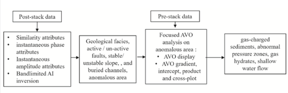
Figure 1 The workflow to integrate the seismic attributes which applicable without well data for preliminary shallow geohazard identification.
Figure 1 shows our proposed work-flow to minimize the above limitations by integrating seismic attributes which are applicable even though there is no well data. It is divided into two main steps:
- The analysis in stack data domain to identify the geological facies, active faults, active slopes and anomalous areas. The attributes to be integrated in the interpretation are the post-stack complex instantaneous (phase and amplitude envelope), vari- ance-based coherence/similarity and bandlimited AI attributes;
- The analysis in the gather data which focused in the anomalous area identified in the first step. The main attributes used here are the AVO cross-plot attributes (gradient, intercept, product) and the main objective is to know the causes of the anomaly.
Application example
To demonstrate the application of the suggested approach, it was applied in the ultra-deep water area with water depths range from 2.0 to 3.2 km (Figure 2a).
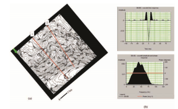
Figure 2 (a) 2D sea-bed depth map, (b) spectrum of wavelet, frequency and phase of the studied interval
The seismic data used in the analysis was processed mainly to image the deeper reservoir targets using the following processing sequence:
- Reformat from SEG-Y to internal format with sampling interval 4 ms
- Geometry update or navigation merger
- Water bottom pick
- Low cut filter 3 Hz/18 dB
- S pike/noise burst in shot domain and direct arrival time noise removal
- Swell noise attenuation and footprint/de-stripping removal
- 1st pass velocity analysis every 500 m x 500 m
- High resolution radon multiple attenuation
- 2nd pass velocity analysis every 250 m x 250 m
- Linear and coherence noise removal and high Resolution Radon Multiple Attenuation
- 3D Kirchhoff Pre-Stack Time Migration
- Normal Moveout Correction using 2nd order velocity
- Muting, stacking, source and streamer static correction
- Random noise attenuation using 3D-FXY Deconvolution
- Time variant filter and scaling
- Output SEGY
There was no additional processing done for the shallow geohazard analysis.
Figures 3 and 4 show the uninterpreted and interpreted amplitude, complex cosine-phase and complex instantaneous amplitude sections of the representative Lines 1 and 2. The anal- ysis focused on the sediments deposited between the F1 primary fault plane and the sea-bed (Figures 3e and 4e). The average Vp and dominant frequency in this deposit are respectively around 1700 m/s and 40 Hz (Figure 2b), which gives the seismic verticalresolution of about 10 m. The seismic data is in zero-phase, reverse polarity (positive reflection coefficient is the centre of the trough) and the Vp of water and seabed are respectively around 1500 m/s and 1700 m/s.
The geological interpretation of the analysed interval in the amplitude sections are difficult, since most reflectors associate with subtle-weak amplitude, very probably because the associ- ated deposits are not well compacted yet and thus their AIs are similar (Figures 3a and 4a). By integrating the complex phaseand instantaneous amplitude attribute, variance-based coherence attribute, and bandlimited inversion, the interpretation of the shallow-geohazard features is much easier as discussed below.
The phase section, which emphasizes layer continuity, facil- itates much easier fault and seismic facies interpretation than the amplitude sections (Figures 3b, 3e, 4b, 4e). Three active lystric normal growth faults, F1, F2 and F3, with the typical character- istics of roll-over anticline and fault dip flattens with depth, are clearly observed.
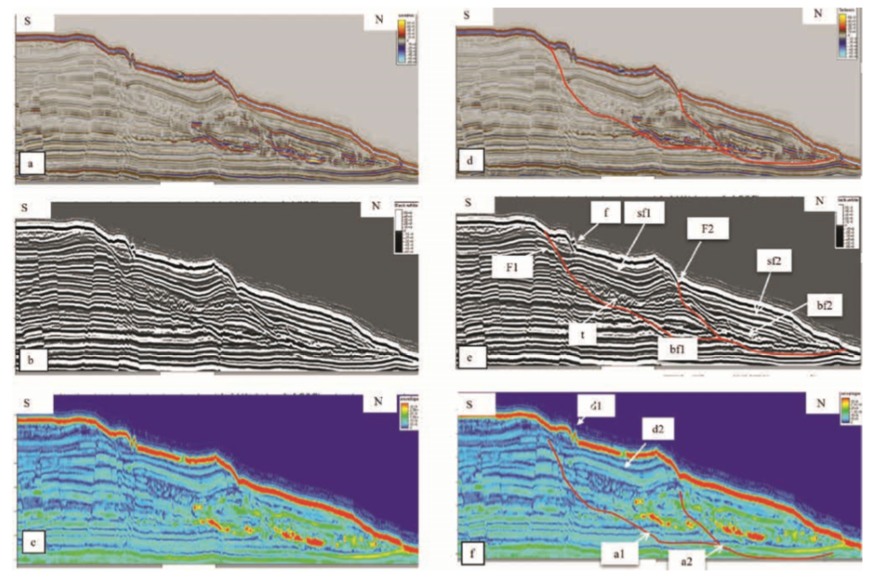
Figure 3 Line 1: Figures 3a to c successively are the un-interpreted amplitude, cosine-phase and amplitude envelope sections. Figures 3d to f are the interpreted ones.
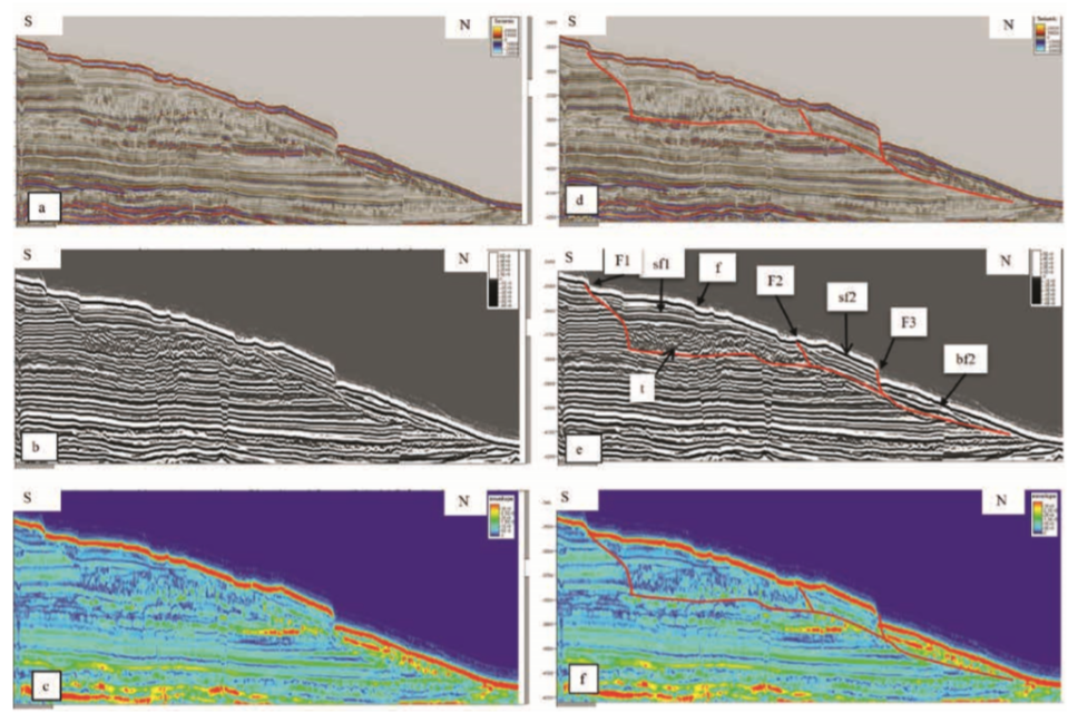
Figure 4 Line 2: Figures 4a to c successively are uninterpreted amplitude, cosine-phase and amplitude envelope sections. Figures 4d to f are the interpreted ones.
Basinward, in front of the F1, a low-stand system tract (LST) package comprises of (from bottom to the top): basin- floor (bf), turbidite (t) and slope-fan (sf) facies, were deposited. The oldest bf facies have typical parallel continuous internal configuration and mounded external shape. Two unitsiden- tifiable: bf1 deposited in front of F1 but behind F2, and bf2 deposited in front of F2.
The t facies have typical slump turbidite sediment charac- teristic: deposited right in front of the F1 steep slope, chaotic internal configuration and sheet external shape. The youngest sffacies have typical characteristics of sheet external shape draping over the underlying sediments. Twounits also identifiable: sf1 deposited in front of F1 with sigmoid configuration, and sf2 deposited in front of F2 with parallel configuration. The sheet drape feature suggests that this facies dominated by fine-grain sediments.
In contrast with the phase section, the amplitude envelope section highlight the amplitude contrast associated with the sea- bed discontinuities (d1 and d2 in Figure 3e) and the bright-spots on the base of the bf facies (a1 and a2 in Figure 3e).
The sea-bed amplitude envelope discontinuities may reflect active fault or unstable slope. A closer look to the phase section shows that the F1, F2, F3 and f1 discontinuities in Figures 3 and 4 connected with a vertical fault consistently displace seabed and underlying sediments; thus, they represent active faults. On the other hand, there is no visible fault connected with d1 discontinu- ity; therefore, it is interpreted as an active slope.
Conclusion
An approach to optimize the application of the 3D conventional seismic data, thus improving its interpretation accuracy, for preliminary shallow geohazard assessment in a deep water area with no well data has been discussed. The approach, done by integrating the seismic attributes applicable without well data, is divided into two steps. The first step is using stack data toidentify the active faults, active slopes, geological facies, and anomalous areas related with SWFS or gas-charged sediments. The integrated attributes are the post-stack complex, similarity, and bandlimited AI attributes. The second step is the pre-stack AVO analysis in the anomalous area identified in the first step, to determine whether the anomaly relates with SWFS or gas-charge sediments.
The approach was tested in the ultra-deep water area with sea-bed ranges from 2.0 to 3.2 km. The 3D conventional data has a good quality and resolution. However, the potential shallow geohazard features are very subtle in this data owing to the weak amplitude of the studied interval. Using the proposed approach, the active faults, unstable slope, geological facies, gas-charged sediments and SWF-associated facies can be identified and mapped. The approach can be used for quick screening and mapping of the potential shallow geohazards prior to a more detailed hazard assessment for safe drilling site selection.
References
- Alamsyah, M.N., Sukmono, S., Marwosuwito, S., Sutjiningsih, W. and Marpaung, L. [2008]. Seismic Reservoir Characterization of South- west Betara Field. The Leading Edge, 27(12), 260-267.
- Campbell, K.J. [1999]. Deepwatergeohazards: How significant are they? The Leading Edge, 18(4), 514-519.
- Castagna, J.P. and Swan, H.W. [1997]. Principles of AVO cross plotting. The Leading Edge, 16(7), 948-956.
- Chopra, S. and Marfurt, K.J. [2007]. Seismic attributes for prospect iden- tification and reservoir characterization, SEG Annual International Meeting, Expanded Abstracts.
- Dutta, N.C., Utech, R.W. and Shelander, D. [2010].Role of 3D seismic for quantitative shallow hazard assessment in deepwater sediments. The Leading Edge, 29(8), 930-942.
- ISO 17776:2000(E). First edition, 2000-10-15.International Organization for Standardization, Geneva, Switzerland.
- Mallick, S. and Dutta, N.C. [2002].Shallow water flow prediction using prestack waveform inversion of conventional 3D seismic data and rock modeling. The Leading Edge, 21(7), 675-680.
- OGP International Associate of Oil and Gas Producers [2011].Guidelines for the conduct of offshore drilling site surveys. IOGP Report 373- 18-1.
- Ostermeier, R.M., Pelletier, J.H., Winker, C.D., Nicholson, J.W., Ram- bow, F.H. and Cowan, K.M. [2002].Dealing with shallow-water flow in the deepwater Gulf of Mexico. The Leading Edge, 21(7), 660-668.
- Russel, B. and Hampson, D. [1991].Comparison of post stack seismic inversion, SEG Annual International Meeting, Expanded Abstracts, 876-878.
- Sukmono, S. [2007]. The Application of Multi-Attributes Analysis in Mapping Lithology and Porosity in the Pematang-Sihapas Groups of Central Sumatra Basin, Indonesia. The Leading Edge, 26(2), 126-131.
- Sukmono, S., Samodra, A., Sardjito and Waluyo, W. [2006]. Integrating Seismic Attributes for Reservoir Characterization in Melandong Field, North West Java Basin, Indonesia, The Leading Edge, 25(5), 532-538.
- Taner, M.T., Koehler, F., and Sheriff, R.E. [1979].Complex seismic trace analysis. Geophysics, 44(6), 1041-1063.